Examples

This chapter shows how to use SACOBRA_Py.

A First Example

This example can be found in first_example.py:

import numpy as np
from cobraInit import CobraInitializer
from cobraPhaseII import CobraPhaseII
from gCOP import COP, show_error_plot

class MyCOP(COP):
    def __init__(self):
        super().__init__()
        self.name = 'first example'
        self.fn = lambda x: np.array([3 * np.sum(x ** 2), 1 - np.sum(x)])
        self.fbest = 1.5
        self.lower = np.array([-5,-5])
        self.upper = np.array([+5,+5])
        self.is_equ = np.array([False])
cop = MyCOP()

cobra = CobraInitializer(None, cop.fn, cop.name, cop.lower, cop.upper, cop.is_equ)

c2 = CobraPhaseII(cobra).start()

print(f"xbest: {cobra.get_xbest()}")
print(f"fbest: {cobra.get_fbest()}")
print(f"final error: {cobra.get_fbest() - cop.fbest}")

show_error_plot(cobra, cop)

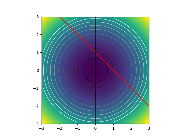
The constraint optimization problem cop consists of a 2-dimensional sphere objective with center at the origin and a linear constraint

\[ g(\vec{x}) = 1 - \sum_i {x_i} \leq 0 \]

which defines the feasible space as the space on and above the straight line passing through \((0,1)\) and \((1,0)\). The true solution is the point of this space closest to the origin, i.e. \(\vec{x}_s = (0.5,0.5)\) with \(f(\vec{x}_s) = 3\vec{x}_s\cdot \vec{x}_s = 1.5\).

A sketch of the COP is shown here (click on image to enlarge):

We initialize SACOBRA_Py with default options, start phase-II-optimization and obtain a very satisfactory result with error < 9 e-13.

G06 with Inequality Constraints

This example can be found in sacobra_ineq.py:

import numpy as np
from gCOP import GCOP, show_error_plot
from cobraInit import CobraInitializer
from cobraPhaseII import CobraPhaseII
from opt.sacOptions import SACoptions
from opt.idOptions import IDoptions
from opt.rbfOptions import RBFoptions
from opt.seqOptions import SEQoptions

G06 = GCOP("G06")

cobra = CobraInitializer(
            G06.x0, G06.fn, G06.name, G06.lower, G06.upper, G06.is_equ, solu=G06.solu,
            s_opts=SACoptions(verbose=1, feval=40, cobraSeed=42,
                              ID=IDoptions(initDesign="LHS", initDesPoints=6),
                              RBF=RBFoptions(degree=2),
                              SEQ=SEQoptions(conTol=1e-7)))
c2 = CobraPhaseII(cobra).start()

show_error_plot(cobra, G06, file="../demo/error_plot_G06.png")

fin_err = np.array(cobra.get_fbest() - G06.fbest)
print(f"final error: {fin_err}")

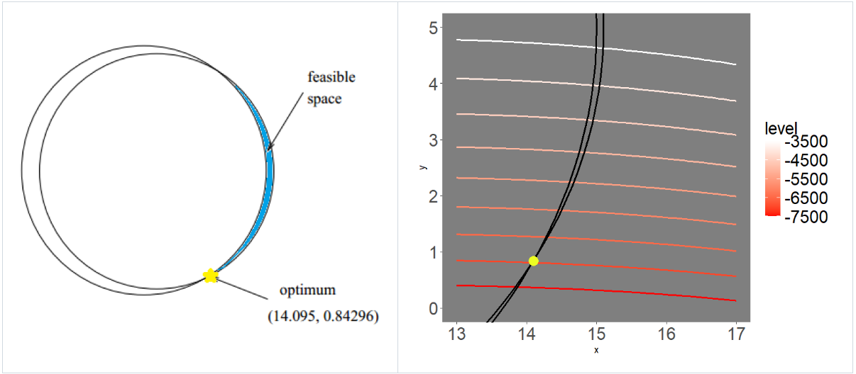
We first load G06 from the G-problem benchmark suite. G06 is a 2D problem with two circular-shaped inequality constraints such that the feasible region is a very narrow crescent-shaped region. A sketch of G06 is shown here (click on image to enlarge):

The object CobraInitializer cobra is initialized with the G06 problem characteristica and its SACoptions are set:

40 function evaluations, seed 42, latin hypercube sampling (LHS) initial design with 6 points, cubic RBF with polynomial tail of degree 2, sequential optimization with constraint violation tolerance of \(10^{-7}\).

Now the optimization is started with CobraPhaseII. The object cobra is modified and enriched by this optimization: The data frames cobra.df and cobra.df2 are extended row-by-row with each iteration and they contain diagnostic information. The dictionary cobra.sac_res is extended as well: For example, the array cobra.sac_res['fbestArray'] has the evolution of the best fitness (objective) value over iterations.

This is used by show_error_plot to display the error curve, which is also saved in PNG file error_plot_G06.png (click on image to enlarge):

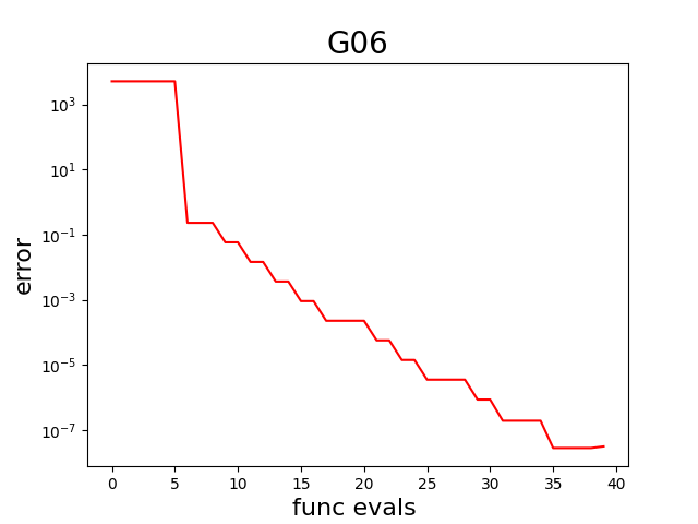
Finally, the final error (difference between the objective value found by the optimizer in the last iteration and the true objective G06.fbest) is computed and printed.

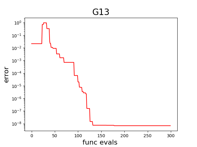
G13 with Equality Constraints

This example can be found in sacobra_equ.py:

import numpy as np
from gCOP import GCOP, show_error_plot
from cobraInit import CobraInitializer
from cobraPhaseII import CobraPhaseII
from opt.equOptions import EQUoptions
from opt.sacOptions import SACoptions
from opt.idOptions import IDoptions
from opt.rbfOptions import RBFoptions
from opt.seqOptions import SEQoptions

G13 = GCOP("G13")

cobra = CobraInitializer(
           G13.x0, G13.fn, G13.name, G13.lower, G13.upper, G13.is_equ, solu=G13.solu,
           s_opts=SACoptions(verbose=1, feval=300, cobraSeed=42,
                             ID=IDoptions(initDesign="LHS", initDesPoints=6*7//2),
                             RBF=RBFoptions(degree=2, rho=2.5, rhoDec=2.0),
                             EQU=EQUoptions(muGrow=100, muDec=1.6, muFinal=1e-7,
                                            refineAlgo="COBYLA"),
                             ISA=ISAoptions2(TGR=1000.0),
                             SEQ=SEQoptions(conTol=1e-7)))
c2 = CobraPhaseII(cobra).start()

show_error_plot(cobra, G13, file="../demo/error_plot_G13.png")

fin_err = np.array(cobra.get_fbest() - G13.fbest)
print(f"final error: {fin_err}")

We first load G13 from the G-problem benchmark suite. G13 is a problem with 3 equality constraints. The rest is very much the same as in the example before, except that the following new options in SACoptions are set:

300 function evaluations,

RBF modeling starts with smoothing factor \(\rho=2.5\) which means approximating RBFs. Parameter \(\rho=2.5\) is exponentially decaying towards 0 with factor rhoDec=2.0. If \(\rho=0\) or if it is very small, then we have interpolating RBFs.

Equality handling with margin \(\mu\) (see EQUoptions), where \(\mu\) is decaying exponentially with factor 1.6 from \(\mu_{init}\) towards \(\mu_{final} = 10^{-7}\), but re-growing every muGrow=100 iterations again to the large initial \(\mu_{init}.\) As refine algo (see EQUoptions) we use “COBYLA” from package nlopt.

As an example we show how ISA is initialized with derived class ISAoptions2 where all the defaults from ISAoptions2 are taken, except that threshold TGR=1000 is set. (ISAoptions would also produce low errors, but ISAoptions0 is not recommended, it would produce much too large errors).

The resulting error curve in PNG file error_plot_G13.png (click on image to enlarge):